X.25 protocol

X.25

X.25 is a protocol suite defined by ITU-T for packet switched communications over WAN (Wide Area Network). It was originally designed for use in the 1970s and became very popular in 1980s. Presently, it is used for networks for ATMs and credit card verification. It allows multiple logical channels to use the same physical line. It also permits data exchange between terminals with different communication speeds.

X.25 has three protocol layers

•  Physical Layer: It lays out the physical, electrical and functional characteristics that interface between the computer terminal and the link to the packet switched node. X.21 physical implementer is commonly used for the linking.
• Data Link Layer: It comprises the link access procedures for exchanging data over the link. Here, control information for transmission over the link is attached to the packets from the packet layer to form the LAPB frame (Link Access Procedure Balanced). This service ensures a bit-oriented, error-free, and ordered delivery of frames.
• Packet Layer: This layer defines the format of data packets and the procedures for control and transmission of the data packets. It provides external virtual circuit service. Virtual circuits may be of two types: virtual call and permanent virtual circuit. The virtual call is established dynamically when needed through call set up procedure, and the circuit is relinquished through call clearing procedure. Permanent virtual circuit, on the other hand, is fixed and network assigned.

Characteristics of X.25

In addition to the characteristics of the packet switched network, X.25 has the following characteristics:

1.      Multiple logical channels can be set on a single physical line

2.      Terminals of different communication speeds can communicate

3.      The procedure for transmission controls can be changed.

The three layers of X.25 interface are as shown in Fig.(a).

• At the physical level X.21 physical interface is being used which is defined for circuit switched data network. At the data link level, X.25 specifies the link access procedure-B (LAP-B) protocol which is a subset of HDLC protocol.

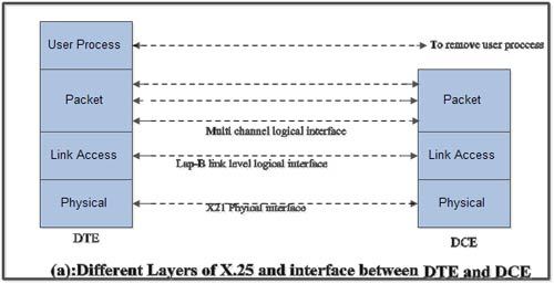
 At the network level (3^rd level), X.25 defines a protocol for an access to packet data subnetwork.

• This protocol defines the format, content and procedures for exchange of control and data transfer packets. The packet layer provides an external virtual circuit service.

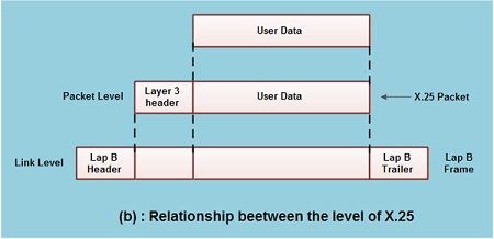
• Fig.(b) shows the relationship between the levels of x'25. User data is passed down to X.25 level 3.

• This data then appends the control information as a header to form a packet. This control .information is then used in the operation of the protocol.

 The entire X.25 packet formed at the packet level is then passed down to the second layer i.e. the data link layer.

The control information is appended at the front and back of the packet forming a LAP-B frame. The control information in LAP-B frame is needed for the operation of the LAP-B protocol.

• This frame is then passed to the physical layer for transmission.

Virtual Circuit Service

• With the X25 packet layer, data are transmitted in packets over external virtual circuits, The virtual circuit service of X25 provides for two types of virtual circuits,

• The virtual circuit service of X25 provides for two types of virtual circuits i.e. "virtual call" and "permanent virtual circuit".

• A virtual call is a dynamically established virtual circuit using a call set up and call clearing procedure.

• A permanent virtual circuit is a fixed, network assigned virtual circuit. Data transfer takes place as with virtual calls, but no call set up or clearing is required.

Prim’s Algorithm( Minimum spanning tree)

Prim’s Algorithm

Prim’s Algorithm also use Greedy approach to find the minimum spanning tree. In Prim’s Algorithm we grow the spanning tree from a starting position. Unlike an edge in Kruskal's, we add vertex to the growing spanning tree in Prim's.

Algorithm Steps:

• Maintain two disjoint sets of vertices. One containing vertices that are in the growing spanning tree and other that are not in the growing spanning tree.
• Select the cheapest vertex that is connected to the growing spanning tree and is not in the growing spanning tree and add it into the growing spanning tree. This can be done using Priority Queues. Insert the vertices, that are connected to growing spanning tree, into the Priority Queue.
• Check for cycles. To do that, mark the nodes which have been already selected and insert only those nodes in the Priority Queue that are not marked.

Consider the example below:

In Prim’s Algorithm, we will start with an arbitrary node (it doesn’t matter which one) and mark it. In each iteration we will mark a new vertex that is adjacent to the one that we have already marked. As a greedy algorithm, Prim’s algorithm will select the cheapest edge and mark the vertex. So we will simply choose the edge with weight 1. In the next iteration we have three options, edges with weight 2, 3 and 4. So, we will select the edge with weight 2 and mark the vertex. Now again we have three options, edges with weight 3, 4 and 5. But we can’t choose edge with weight 3 as it is creating a cycle. So we will select the edge with weight 4 and we end up with the minimum spanning tree of total cost 7 ( = 1 + 2 +4).

Time Complexity:
The time complexity of the Prim’s Algorithm is $O((V+E)logV)$ because each vertex is inserted in the priority queue only once and insertion in priority queue take logarithmic time.

Kruskal’s Algorithm( Minimum Spanning Tree)

Kruskal’s Algorithm

Kruskal’s Algorithm builds the spanning tree by adding edges one by one into a growing spanning tree. Kruskal's algorithm follows greedy approach as in each iteration it finds an edge which has least weight and add it to the growing spanning tree.

Algorithm Steps:

• Sort the graph edges with respect to their weights.
• Start adding edges to the MST from the edge with the smallest weight until the edge of the largest weight.
• Only add edges which doesn't form a cycle , edges which connect only disconnected components.

So now the question is how to check if $2$ vertices are connected or not ?

This could be done using DFS which starts from the first vertex, then check if the second vertex is visited or not. But DFS will make time complexity large as it has an order of $O(V+E)$ where $V$ is the number of vertices, $E$ is the number of edges. So the best solution is "Disjoint Sets":
Disjoint sets are sets whose intersection is the empty set so it means that they don't have any element in common.

Consider following example:

In Kruskal’s algorithm, at each iteration we will select the edge with the lowest weight. So, we will start with the lowest weighted edge first i.e., the edges with weight 1. After that we will select the second lowest weighted edge i.e., edge with weight 2. Notice these two edges are totally disjoint. Now, the next edge will be the third lowest weighted edge i.e., edge with weight 3, which connects the two disjoint pieces of the graph. Now, we are not allowed to pick the edge with weight 4, that will create a cycle and we can’t have any cycles. So we will select the fifth lowest weighted edge i.e., edge with weight 5. Now the other two edges will create cycles so we will ignore them. In the end, we end up with a minimum spanning tree with total cost 11 ( = 1 + 2 + 3 + 5).

Time Complexity:
In Kruskal’s algorithm, most time consuming operation is sorting because the total complexity of the Disjoint-Set operations will be $O(ElogV)$, which is the overall Time Complexity of the algorithm.

Minimum Spanning Tree

What is a Spanning Tree?

Given an undirected and connected graph $G=(V,E)$, a spanning tree of the graph $G$ is a tree that spans $G$ (that is, it includes every vertex of $G$) and is a subgraph of $G$ (every edge in the tree belongs to $G$)

What is a Minimum Spanning Tree?

The cost of the spanning tree is the sum of the weights of all the edges in the tree. There can be many spanning trees. Minimum spanning tree is the spanning tree where the cost is minimum among all the spanning trees. There also can be many minimum spanning trees.

Minimum spanning tree has direct application in the design of networks. It is used in algorithms approximating the travelling salesman problem, multi-terminal minimum cut problem and minimum-cost weighted perfect matching. Other practical applications are:

1. Cluster Analysis
2. Handwriting recognition
3. Image segmentation     

There are two famous algorithms for finding the Minimum Spanning Tree:

Kruskal’s Algorithm

Kruskal’s Algorithm builds the spanning tree by adding edges one by one into a growing spanning tree. Kruskal's algorithm follows greedy approach as in each iteration it finds an edge which has least weight and add it to the growing spanning tree.

Prim’s Algorithm

Prim’s Algorithm also use Greedy approach to find the minimum spanning tree. In Prim’s Algorithm we grow the spanning tree from a starting position. Unlike an edge in Kruskal's, we add vertex to the growing spanning tree in Prim's.

Routing Algorithm

Routing Algorithm

Routing is process of establishing the routes that data packets must follow to reach the destination. In this process, a routing table table is created which contains information regarding routes which data packets follow. Various routing algorithm are used for the purpose of deciding which route an incoming data packet needs to be transmitted on to reach destination efficiently.

Classification of Routing Algorithms: The routing algorithms can be classified as follows:

1.    Adaptive Algorithms –
These are the algorithms which change their routing decisions whenever network topology or traffic load changes. The changes in routing decisions are reflected in the topology as well as traffic of the network. Also known as dynamic routing, these make use of dynamic information such as current topology, load, delay, etc. to select routes. Optimization parameters are distance, number of hops and estimated transit time.

2.     Non-Adaptive Algorithms –
These are the algorithms which do not change their routing decisions once they have been selected. This is also known as static routing as route to be taken is computed in advance and downloaded to routers when router is booted.

**Performance criteria of routing algorithm

The variables are generally known as routing metrics and can include the following:

·          Hops: The number of intermediate routers between a given network and the local router 

·           Latency: The time delay in processing a packet through the router or over a given route 

• Congestion: The length of the packet queue at the incoming port of the router 
• Load: The processor use at the router or the number of packets per second that it is currently processing 
• Bandwidth: The available capacity of a route to support network traffic; decreases as network traffic increases 
• Reliability: The relative amount of downtime that a particular router might experience because of malfunctions 
• Maximum Transmission Unit (MTU): The largest packet size that the router can forward without needing to fragment the packet 

**Routing Strategies :

• Fixed Routing
• Flooding
• Dynamic Routing
• Random Routing
• Flow-based Routing                                                                                                              

Fixed Routing –
·       A route is selected for each source and destination pair of node in the network.

·       The route is fixed ; changes only if the topology of the network changes.

Fixed Routing : Example (1)

·       Figure – A simple packet switching network with six nodes (routers)

Figure – Central routing table based on least cost path algorithm

• A Central routing matrix is created based on the least-cost path which is stored in the network control center
• The matrix, shows for each source-destination of the route , the identity of the next node on the route.
• Drawback: If the network control center fails, then everything will collapse. Hence it is not reliable.
• Fixed Routing : Example (2)
• 

Figure – Routing table stored in different nodes of the network

• Routing Table is created for each node. This is called a distributed routing algorithm
• Routing table can be created using least-min path or min-hop reach method. Two famous path algorithms
  1. Dijkstra Algorithm
  2. Bellman Ford Algorithm

Advantages –

• Simple
• Works well in reliable network with stable load in reliable network
• Same for virtual circuit and datagram

Disadvantages –

• Lack of flexibility
• Doesn’t react to failure or network congestion

Reference: https://www.geeksforgeeks.org/

Mergesort

Merge sort is a divide-and-conquer algorithm based on the idea of breaking down a list into several sub-lists until each sublist consists of a single element and merging those sublists in a manner that results into a sorted list.

Idea:

• Divide the unsorted list into N sublists, each containing 1 element.
• Take adjacent pairs of two singleton lists and merge them to form a list of 2 elements. N will now convert into N/2 lists of size 2.
• Repeat the process till a single sorted list of obtained.

While comparing two sublists for merging, the first element of both lists is taken into consideration. While sorting in ascending order, the element that is of a lesser value becomes a new element of the sorted list. This procedure is repeated until both the smaller sublists are empty and the new combined sublist comprises all the elements of both the sublists.

As one may understand from the image above, at each step a list of size M is being divided into 2 sublists of size M/2, until no further division can be done. 

To understand better, consider a smaller array A containing the elements (9,7,8).

At the first step this list of size 3 is divided into 2 sublists the first consisting of elements (9,7) and the second one being (8).

 Now, the first list consisting of elements (9,7) is further divided into 2 sublists consisting of elements (9) and (7) respectively.

As no further breakdown of this list can be done, as each sublist consists of a maximum of 1 element, we now start to merge these lists.

 The 2 sub-lists formed in the last step are then merged together in sorted order using the procedure mentioned above leading to a new list (7,9). Backtracking further, we then need to merge the list consisting of element (8) too with this list, leading to the new sorted list (7,8,9).

An implementation has been provided below :

 void merge(int A[ ] , int start, int mid, int end) {

 //stores the starting position of both parts in temporary variables.

int p = start ,q = mid+1;

int Arr[end-start+1] , k=0;

for(int i = start ;i <= end ;i++) {

    if(p > mid)      //checks if first part comes to an end or not .

       Arr[ k++ ] = A[ q++] ;

   else if ( q > end)   //checks if second part comes to an end or not

       Arr[ k++ ] = A[ p++ ];

   else if( A[ p ] < A[ q ])     //checks which part has smaller element.

      Arr[ k++ ] = A[ p++ ];

   else

      Arr[ k++ ] = A[ q++];

 }

  for (int p=0 ; p< k ;p ++) {

   /* Now the real array has elements in sorted manner including both

        parts.*/

     A[ start++ ] = Arr[ p ] ;                         

  }

}

Here, in merge function, we will merge two parts of the arrays where one part has starting and ending positions from start to mid respectively and another part has positions from mid+1 to the end.

A beginning is made from the starting parts of both arrays. i.e. p and q. Then the respective elements of both the parts are compared and the one with the smaller value will be stored in the auxiliary array (Arr[ ]). If at some condition ,one part comes to end ,then all the elements of another part of array are added in the auxiliary array in the same order they exist.

Now consider the following 2 branched recursive function :

   void merge_sort (int A[ ] , int start , int end )

   {

           if( start < end ) {

           int mid = (start + end ) / 2 ;           // defines the current array in 2 parts .

           merge_sort (A, start , mid ) ;                 // sort the 1st part of array .

           merge_sort (A,mid+1 , end ) ;              // sort the 2nd part of array.

         // merge the both parts by comparing elements of both the parts.

          merge(A,start , mid , end );  

   }                   

}

Time Complexity:
The list of size N is divided into a max of logN parts, and the merging of all sublists into a single list takes O(N) time, the worst case run time of this algorithm is O(NLogN)